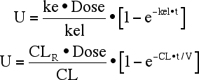
Equation 5.3.1 Cumulative Amount excreted into Urine versus Time
return to the Course index
previous | next
The linear plot of cumulative amount excreted into urine as unchanged drug versus time is shown below. Notice that the value of U∞ is NOT EQUAL to the dose, it is somewhat less than dose, unless all of the dose is excreted into urine as unchanged drug. The remaining portion of the dose should be found as metabolites and from other routes of excretion.
The equation for the cumulative amount excreted versus time is shown below in Equation 5.3.1.
Equation 5.3.1 Cumulative Amount excreted into Urine versus Time
This translates into the plot shown in Figure 5.3.1. Notice that the total amount excreted as unchanged drug, U∞, is less than the dose administered in this plot.

Figure 5.3.1 Linear Plot of U versus Time showing Approach to U∞ not equal to DOSE
Click on the figure to view the interactive graph
Cumulative amount excreted plots are basically descriptive in nature. At most, you can get a general sense of how much drug is excreted, an estimate of U∞ and an approximate estimate of t1/2.
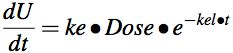
Equation 5.3.2 Rate of Excretion of Unchanged Drug into Urine
Since urine data is collected over an interval of time the data is represented as ΔU rather than dU. Also, since ΔU is collected over a discrete time interval the time point for this interval should be the midpoint of the interval, tmidpoint. Equation 5.3.2 can be replaced by Equation 5.3.3 to better represent the data collected. It may look like a strange way of plotting the data, but actually it's quite convenient to use because urine data results are collected as an amount of drug excreted during a time interval. The amount excreted is the product of the volume of urine voided and the concentration of drug in the sample. This is a rate measurement.
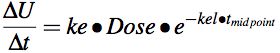
Equation 5.3.3 Rate of Excretion of Unchanged Drug versus midpoint time
Taking the ln of both sides gives Equation 5.3.4, an equation for a straight line. Plotting ln[ΔU/Δt] versus timemidpoint provides kel from the slope and ke from the intercept divided by the Dose
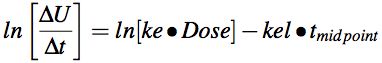
Equation 5.3.4. Natural log of Rate of Excretion versus Time
Note: The intercept (on semi-log graph paper) is ke • DOSE.

Figure 5.3.2. Semi-log Plot of ΔU/Δt versus Timemidpoint Showing Slope = - kel
with fe = 0.75, kel = 0.2 hr-1; ke = 0.15 hr-1
Click on the figure to view the interactive graph
Rate of excretion plots can be very useful in the determination of the parameters such as kel, ke and fe. There can be a little more scatter that with the ARE plot, below. Analysis of 'real' data may show considerable scatter in the rate of excretion plot. Thus, positioning the straight line on a semi-log plot may be difficult. In practical terms it is difficult to get a lot of early times points unless the subjects are catheterized and even then early times may be difficult to interpret. This means that this method can be difficult to use with drugs which have short half-lives. However, a significant advantage of the rate of excretion plot is that each data point is essentially independent, especially if the bladder is fully voided for each sample. A missed sample or data points is not critical to the analysis.NOTE: This plot is rate of excretion versus midpoint of the collection interval, time.
Equation 5.3.5 Cumulative amount excreted versus time
Equation 5.3.6 Total Amount Excreted as Unchanged Drug, Uinfinity
Equation 5.3.5 can be rewritten in terms of Uinfinity.
Equation 5.3.7 Cumulative amount excreted versus time
Equation 5.3.8 Cumulative amount excreted versus time
Rearranging Equation 5.3.8 gives Equation 5.3.9.
Equation 5.3.9 Amount Remaining to be Excreted as Unchanged Drug versus Time
Equation 5.3.10 Ln(ARE) versus time
where
Equation 5.3.11 U∞
Thus:
Equation 5.3.12 ARE versus time
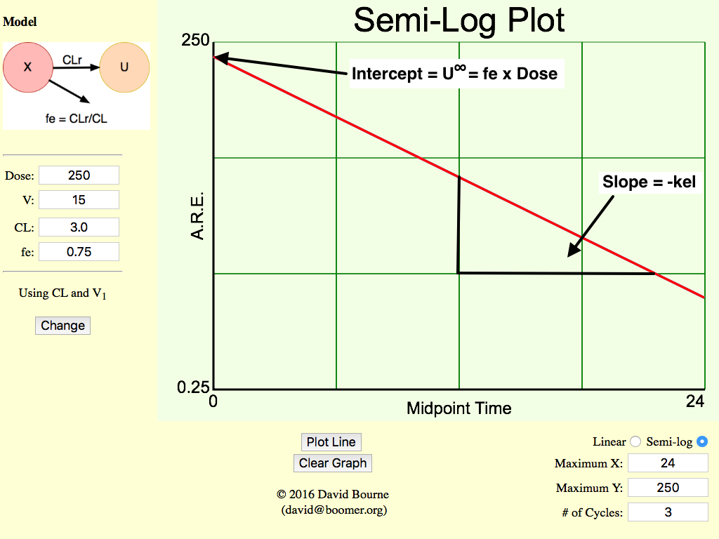
Figure 5.3.3 Semi-log Plot of ARE versus time
Click on the figure to view the interactive graph
Amount remaining to be excreted (ARE) plots use the U∞ value to estimate each data point. Error in any data is accumulated into U∞ and thus each ARE value. This can lead to curved lines (instead of the expected straight lines) or an inability to use the method (with a missing sample). With good data these plots may be somewhat smoother.
![]()
Material on this website should be used for Educational or Self-Study Purposes Only
Copyright © 2001 - 2026 David W. A. Bourne (david@boomer.org)
 | An iPhone app that facilitates the geotagging of Bird Count stops and the return to the same stops during the next and subsequent Bird Count sessions |
|