return to the Course index
previous | next
The superposition principle can be used when all the disposition processes are linear. The disposition processes are distribution, metabolism and excretion (DME). That is, the processes that occur after the drug is absorbed. Thus, the superposition principle can be used when the DME processes are linear or first-order. According to this approach concentrations after multiple doses can be calculated by adding together the concentrations from each dose. Also, doubling the dose will result in the concentrations at each time doubling. This is not true when disposition processes are non-linear.
For example, calculate drug concentration at 24 hours after the first dose of 200 mg. The second dose of 300 mg was given at 6 hours and the third dose of 100 mg at 18 hours. The apparent volume of distribution is 15 L and the elimination rate constant is 0.15 hr-1.
The concentration from the first dose at 24 hours after the administration of the first dose
The concentration from the second dose at 24 hours after the administration of the first dose
The concentration from the third dose at 24 hours after the administration of the first dose
![]()
The total concentration from all three doses at 24 hours after the administration of the first dose. This method involved calculating the contribution from each dose at a time 24 hours after the first dose.
The result of this calculation is shown graphically in Figure 15.5.1.

Figure 15.5.1 Drug Concentration after Three IV Bolus Doses
Click on the figure to view the interactive graph
Another approach is to work through the dosing regimen dose by dose.
Total drug concentration just after the first dose
![]()
Total drug concentration just before the second dose
Total drug concentration just after the second dose
![]()
Total drug concentration just before the third dose
Total drug concentration just after the third dose
![]()
Total drug concentration 6 hours after the third dose. This answer can also be calculated using an Excel spreadsheet illustrating the superposition principle.
Click on the figure
to download and use this Excel spreadsheet or here for a Numbers version
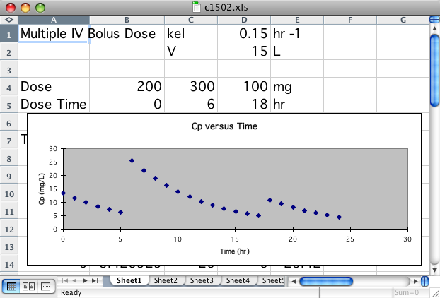
Prior to this Chapter the calculations we have looked at consider that the dosing intervals are quite uniform, however, commonly this ideal situation is not adhered to completely.
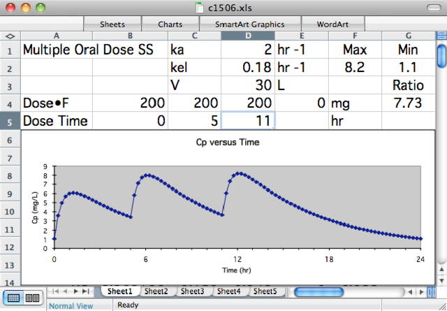
Dosing three times a day may be interpreted as take with meals, the plasma concentration may then look like the plot in Figure 60. The ratio between Cpmax and Cpmin is seven fold (8.2/1.1 = 7.45) in this example.
Figure 15.5.3 Cp versus Time during Dosing at 8 am, 1 pm, and 7 pm
Click on the figure to view the interactive graph
However this regimen may be acceptable if
1) the drug has a wide therapeutic index
2) there is no therapeutic disadvantage to low overnight plasma concentrations, e.g., analgesic if patient stays asleep.
This regimen can be explored further using an Excel spreadsheet illustrating the superposition principle.
Click on the figure
to download and use this Excel spreadsheet
Other practice problems involving the calculation of Cp at three times during a uniform dosing interval with Linear or Semi-log graphical answers or calculation of Cp at three times during a non-uniform dosing interval with Linear or Semi-log graphical answers
Material on this website should be used for Educational or Self-Study Purposes Only
Copyright © 2001 - 2026 David W. A. Bourne (david@boomer.org)
 | A tvOS app which presents a collection of video tutorials related to Basic Pharmacokinetics and Pharmacy Math |
|